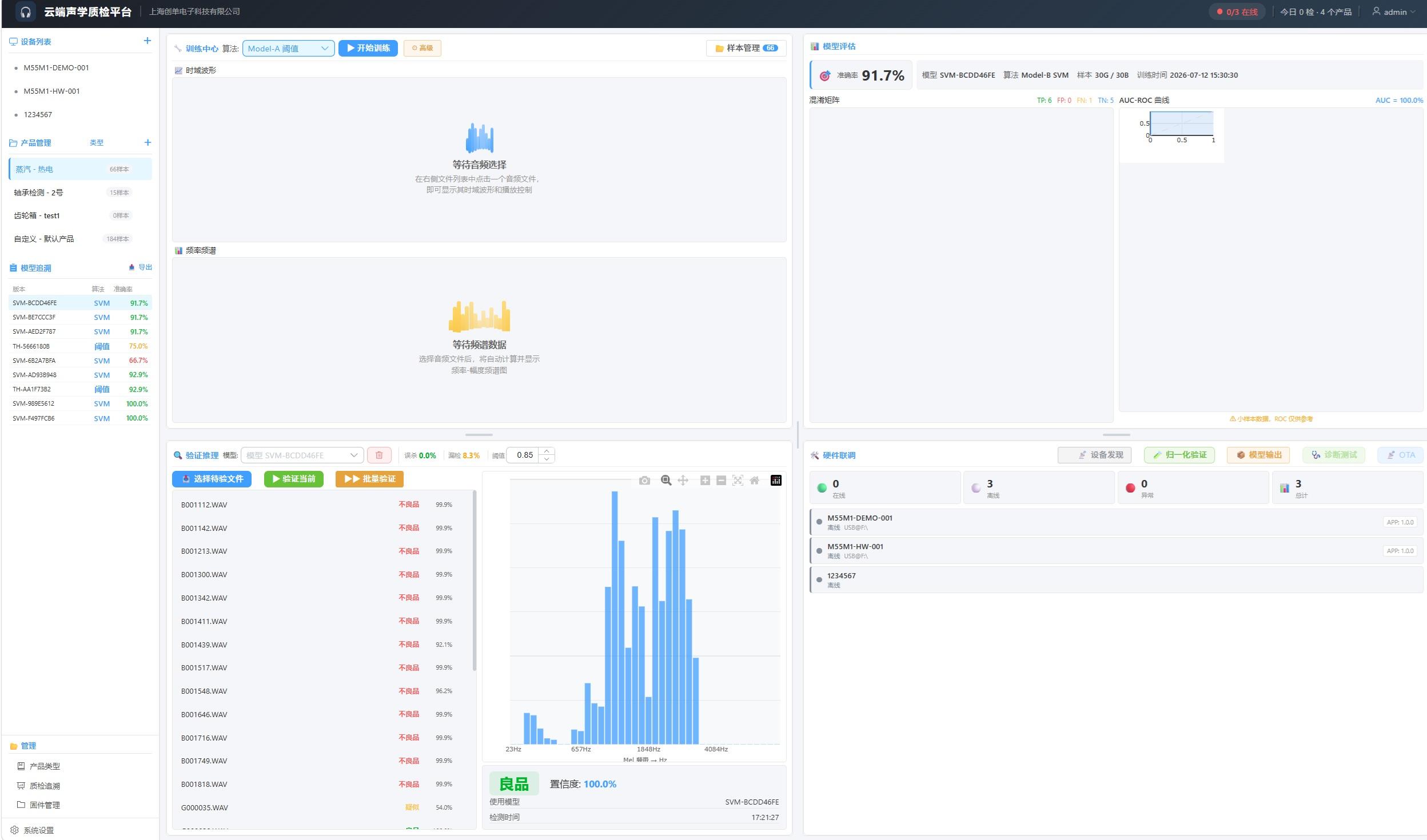
A model that scores 98% on a lab laptop drops to 70% once it runs on a production-line MCU. If you have shipped industrial acoustic AI, that gap is probably familiar.
The awkward part is that the model is not the problem. Not one byte of the model weights has changed. The only thing that changed is that the feature extraction code was rewritten from Python into C.
In machine vision this gap is usually survivable. The preprocessing chain — resize, normalize — is fairly standardized, and the network downstream can absorb the difference between floating-point and fixed-point.
Acoustics is different. The feature extraction chain in acoustic AI is much longer than in vision, and much more fragile.
01 Why Acoustics Is Especially Fragile
A vision model receives raw, or lightly processed, pixels. Most of the feature learning is delegated to the network itself.
An acoustic model receives hand-designed features: FFT spectra, Mel filter bank energies, MFCC cepstral coefficients. Before those features ever reach a classifier, they have already passed through four or five mathematical transformations.
raw waveform → framing + windowing → FFT → Mel filter bank → log compression → DCT → MFCC
Each transformation is implemented slightly differently on each platform. Taken alone, each deviation may be only 1–3%. But these deviations accumulate layer by layer, and after the non-linear mapping of the classifier, they can flip the final verdict outright.
A sample that should be judged Pass drifts across the decision boundary and becomes Fail. That is the technical root cause of "stunning in the demo, broken on the line."
Put simply: if the front-end features do not match, no amount of algorithm downstream will help. Garbage in, garbage out.
02 Four Compounding Sources of Deviation
Take the classic pairing — training with Librosa in Python, inferring with CMSIS-DSP in C. Deviation enters at four levels.
Deviation 1: FFT implementation
The Python side typically uses a real-valued FFT with a zero-padding strategy; the C side often uses a fixed-point Q-format FFT. The two differ by 1–3% in spectral magnitude.
That looks small. But it is the input to every subsequent computation, so it propagates all the way to the end.
Deviation 2: The Mel filter bank standard split
This is the easiest trap to fall into and the easiest to overlook.
There are two mainstream formulations of the Mel filter bank:
-HTK — Librosa's default. Triangular filters on a uniformly spaced Mel scale.
-Slaney — the default in CMSIS-DSP and several embedded libraries. The normalization differs.
The band weights produced by the two differ by a systematic offset. Note the key word: systematic. This is not random error, so it does not cancel out statistically. It pushes the features consistently in one direction.
Deviation 3: DCT coefficient precision and accumulation order
The last step of MFCC is a DCT over the log Mel energies.
Python runs in double precision; C runs in single precision or fixed point, and often reorders the multiply-accumulate sequence for speed. Floating-point addition is not associative, so a different accumulation order produces a different mantissa — and this shows up most strongly in the higher MFCC dimensions.
Which is unfortunate, because the higher MFCC dimensions are exactly what discriminates many abnormal-noise defects: electromagnetic whine, high-frequency friction.
Deviation 4: Log10 implementation precision
When taking the logarithm of Mel energies, Python uses a high-precision math library implementation, while the C side often uses a lookup table or polynomial approximation for speed.
On low-energy bands the difference is amplified, because the log function is steep there — a tiny input difference produces a large output difference. The result is S/N distortion in the low-energy bands, which are precisely the bands that carry faint defect signatures.
03 How to Align: Four Engineering Constraints
The goal is not "make the error as small as possible." It is eliminate the degrees of freedom that create the error in the first place.
These four measures have held up in production:
Constraint 1: Hardcode the Mel filter bank
Stop letting each side compute Mel weights from its own formula. Instead:
Export the Mel weight matrix from the C side; have Python load that exact same data.
This removes the HTK-versus-Slaney question entirely. Both sides use the same table, so there is no longer a "which standard does each side use" problem.
Constraint 2: Put DCT in a lookup table
Precompute the DCT coefficient table:
-C side: table lookup for the multiply-accumulate
-Python side: np.dot with the same table
This removes the precision difference caused by accumulation order. Both sides perform the same matrix operation, so identical input yields identical output.
Constraint 3: Unify Log10 precision
Implement a table-based Log10 on the C side; have Python emulate the same table with np.interp.
The point is using the same table, not "each side implements a high-precision version." Only when the interpolation matches does the compression behavior on low-energy bands match exactly.
Constraint 4: Make the FFT instance global
Avoid re-initializing the FFT instance on every call. Different initializations can introduce different padding strategies and with them non-determinism. With a global instance, every FFT runs under identical configuration.
04 How to Validate: Compare Dimension by Dimension, Not Final Accuracy
This is where many teams go wrong — they validate feature alignment using final accuracy.
The problem is that accuracy is a blunt instrument. The features may already have drifted, but as long as the drift has not pushed samples across the decision boundary in bulk, accuracy drops only a point or two and nothing looks wrong. The problem surfaces all at once later, on the production line, when critical samples show up.
The correct approach is to compare the feature vector dimension by dimension:
1. Prepare one identical test signal (using both a 1 kHz sine and broadband noise is recommended, to exercise narrowband and wideband response separately)
2. Run the full feature extraction chain on the Python side and on the C side
3. Emit the intermediate feature vector and compare the values dimension by dimension
For an 88-dimensional acoustic feature, compare each dimension and then compute the mean error across dimensions. A workable engineering target is under 0.05% error on every dimension.
What this looks like in practice
The table below is from a real alignment run on the same motor anomaly recording, using the method above:
Test signal | MFCC mean error | MFCC std error | Dimensions passing
1 kHz sine | <0.01% | <0.02% | 88/88
Broadband noise | <0.05% | <0.08% | 88/88
Real motor sound | <0.03% | <0.06% | 87/88
Note the last row. 87 out of 88 — not 88 out of 88.
That single dimension is the reason this article exists. An aggregate accuracy figure would have hidden it completely: one dimension out of 88 moves the top-line number by a fraction of a percent, and everything looks fine. But that dimension is sitting close to the boundary, and on a production line, the samples that matter most are the ones sitting close to the boundary.
This is also why we do not describe the result as "zero degradation." It is not. It is a measured, bounded, and monitored residual — which is a far more useful thing to have than a claim.
05 A Checklist You Can Actually Run
If you are about to deploy acoustic AI to an edge target, work through these in order:
Check | Common failure | Fix
Mel filter standard | Python uses HTK, C uses Slaney | Export the weight matrix from one side; load the same data on both
DCT implementation | Double vs single precision, different accumulation order | Precompute a table; use the same table on both sides
Log implementation | Math library vs fixed-point approximation | Unify on a table lookup with matching interpolation
FFT initialization | Re-initialized on every call | Globalize the instance; fix the padding strategy
Window function | Hann defined as periodic vs symmetric | Define it explicitly and pin it on both sides
Normalization parameters | Mean and variance computed separately on each side | Freeze them on the training side and write them into firmware
Validation method | Watching final accuracy only | Switch to dimension-by-dimension comparison of intermediate features
Two of these are the ones that get missed most often. Window function definition: Hann has both periodic and symmetric definitions, differing by one sample in length, which is not negligible for short frames. Normalization parameters: if each side computes its own mean and variance, even a slight difference in data distribution causes a mismatch.
Closing
Cross-platform feature alignment is not an algorithm problem. It is a problem of engineering discipline.
What it takes is not a cleverer model, but treating "the two ends must agree" as a non-negotiable line and enforcing it down to the implementation of every layer in the feature extraction chain. This is why teams with strong algorithmic capability still stall at industrial deployment — the academic curriculum does not include this subject.
Get it right, though, and the payoff is long-lived: no deployment regression when you iterate the model, no pointless retraining during on-site commissioning, and a materially shorter path from project start to a running line.
The alignment method described here has been validated on multiple production-line deployments on ARM Cortex-M55 with CMSIS-DSP, with per-dimension error below 0.05% across an 88-dimensional acoustic feature set.
What it takes is not a cleverer model, but treating "the two ends must agree" as a non-negotiable line and enforcing it down to the implementation of every layer in the feature extraction chain. This is why teams with strong algorithmic capability still stall at industrial deployment — the academic curriculum does not include this subject.
Get it right, though, and the payoff is long-lived: no deployment regression when you iterate the model, no pointless retraining during on-site commissioning, and a materially shorter path from project start to a running line.
The alignment method described here has been validated on multiple production-line deployments on ARM Cortex-M55 with CMSIS-DSP, with per-dimension error below 0.05% across an 88-dimensional acoustic feature set.